Shell-Based Honeycomb Modelling for Impact Protection in Projectile Electronics
Hi! At the beginning of my 2nd year pursuing a Bachelor’s in Mechanical Engineering at IIT Roorkee, I took up a project under Prof. Avinash Kumar Swain, along with my great friend Garv Jain. Now that it’s completed, I thought writing a blog would be the best way to document our learnings — so here it is!
First of all, I would like to express my heartfelt gratitude to our mentor, Mr. Darshan (PhD student, IITR), for always being there to guide us throughout this journey.
Here’s to link of my GitHub repo containing relevant codes: honeycomb_lsdyna
Slight Introduction
Suppose you want your projectile to hit a target buried under 4–5 layers of thick concrete walls. One of the most mission-critical factors is the survivability of the projectile’s electronics — especially the fuse. Repeated impacts often damage or disturb these internal electronics, leading to mission failure.
The solution? Enclose the electronics inside a robust layer of shock-absorbing material. One of the most promising structures for this purpose — known for its high strength-to-weight ratio — is the honeycomb!
Honeycomb structures are renowned for their excellent energy absorption, lightweight nature, and ability to undergo large deformations while maintaining integrity.
FEA for Honeycomb Impact Simulation
Physical tests for every design iteration are impractical. This is where Finite Element Analysis (FEA) shines. It allows engineers to simulate and refine designs rapidly.
There are two main ways to simulate high strain-rate deformation of honeycomb structures in LS-DYNA:
1. Predefined Honeycomb Material Model
- Uses a simple solid block and applies a mathematical model like
MAT_126 (MODIFIED_HONEYCOMB). - Pros: Saves time and computational cost.
- Cons: Lower accuracy; cannot handle unusual configurations well; poor local deformation detail.
2. Accurate Mesh of True Geometry
- Fully models the honeycomb geometry using shell elements.
- Pros: High accuracy; detailed stress and crush analysis.
- Cons: Computationally expensive.
Our Objective
We aimed to develop an accurate numerical model using the true honeycomb geometry, validated under high strain-rate conditions. We chose LS-DYNA over ANSYS Workbench for its explicit dynamics capabilities and fine control via LS-PrePost.
To validate, I replicated results from:
Stanczak M, Fras T, Blanc L, Pawlowski P, Rusinek A. Blast-Induced Compression of a Thin-Walled Aluminum Honeycomb Structure—Experiment and Modeling. Metals. 2019; 9(12):1350. DOI
The Paper
The authors detonated a C4 charge and used an explosion driven shock tube (EDST) to transfer the shock wave towards the test subject. Use of EDST allows enhanced repeatability and stability of results than free-air detonation based experiments. I used the 50 g blast load and 53 cell honeycomb model results to verify our numerical study.
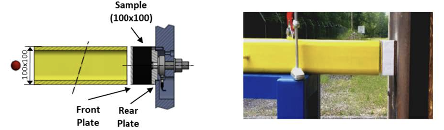 Figure 1: EDST experimental setup
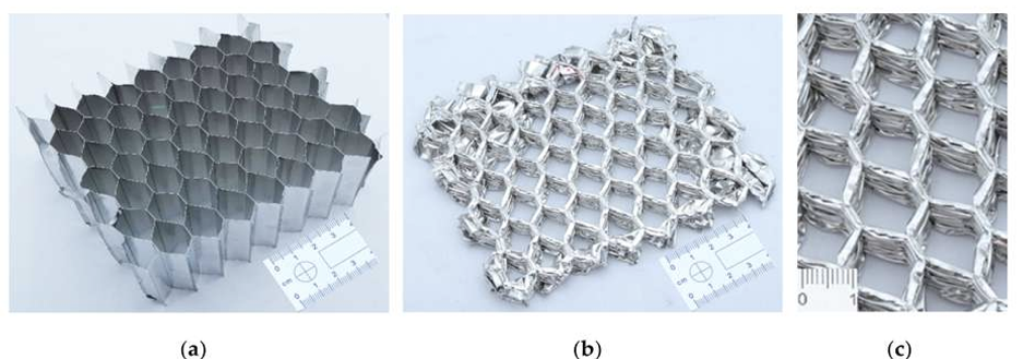 Figure 2: A 53-cell honeycomb structure: (a) non-deformed and (b,c) fully compressed.
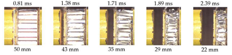 Figure 3: Subsequent frames depicting compression of the honeycomb
 Figure 4: Comparison between the blast load profiles and the structural responses
Methodology
1.1 Model Setup
I first attempted to employ a solid mesh using tetrahedral elements by first modelling the geometry in SolidWorks → IGES → LS-PrePost but faced massless node errors due to poor mesh quality. Eventually, I learned that with a 0.07 mm sheet thickness, shell elements were the right choice.
Key learning: Use shell elements for thin honeycomb walls!
Here’s a video I made for making a shell-based honeycomb mesh:
(Make a honeycomb shell in LS-DYNA)
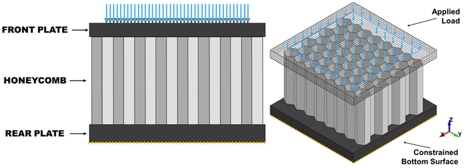
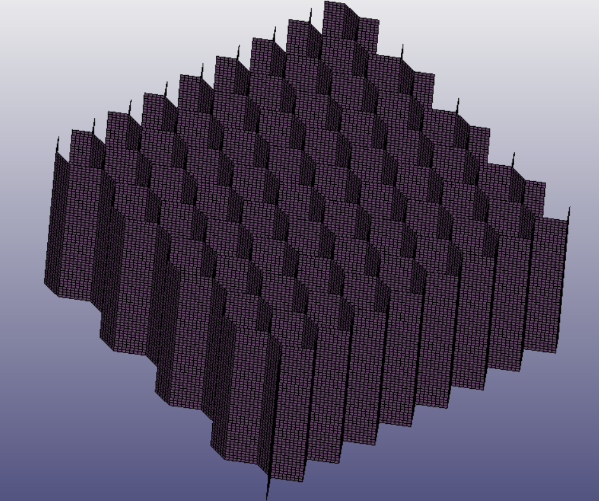 Figure: Honeycomb mesh in Ls-DYNA
Mesh Challenges:
- Determining the right element size took time.
- Mesh convergence was limited due to complex geometry.
- Heuristic Shape Criterion Error required careful aspect ratios.
1.2 Material Properties
For aluminum and steel plates, I used MAT_SIMPLIFIED_JOHNSON_COOK (098). LS-DYNA lacks a built-in unit system, so consistency was crucial.
1.3 Blast Loading
The EDST blast load was applied via LOAD_NODE_SET over an 80×80 mm² area on the front plate, using time-varying force data from the paper.
1.4 Contacts
CONTACT_AUTOMATIC_SURFACE_TO_SURFACEfor plate–honeycomb interfaces.CONTACT_AUTOMATIC_SINGLE_SURFACEfor honeycomb self-contact.
1.5 Simulation Setup
- Bottom of back plate: fixed using
BOUNDARY_SPC. ENDTIME = 4 msbased on experimental Force–Time graphs.TSSFAC = 0.5for stability in explicit integration.
Results & Discussion
Force Reduction
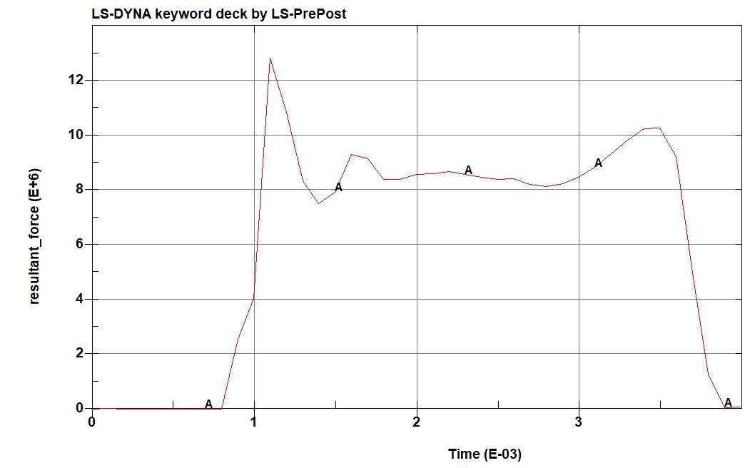 Figure: Resultant Force (mN) vs Time (ms)
The simulation showed the honeycomb reduced the peak force from ~79 kN to ~13 kN — a drop of 83.5%.
RMSE
I digitised the experimental and true plots, converted them to CSV and compared using Jupyter Notebooks:
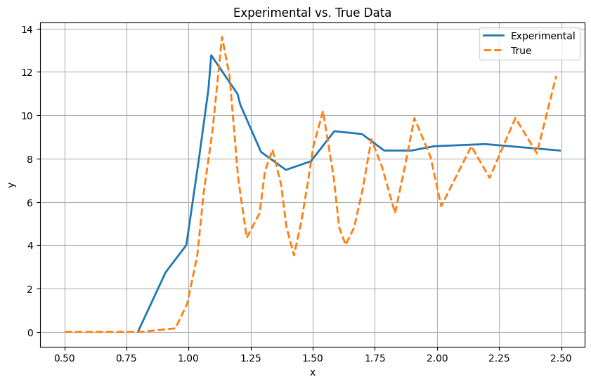
The Relative- RMSE (Root Mean Square Error) came out to be -> 0.1895 i.e., (18.95%)
Not bad, but resolution mismatches and slight geometry differences contributed to error.
Final Crush Height
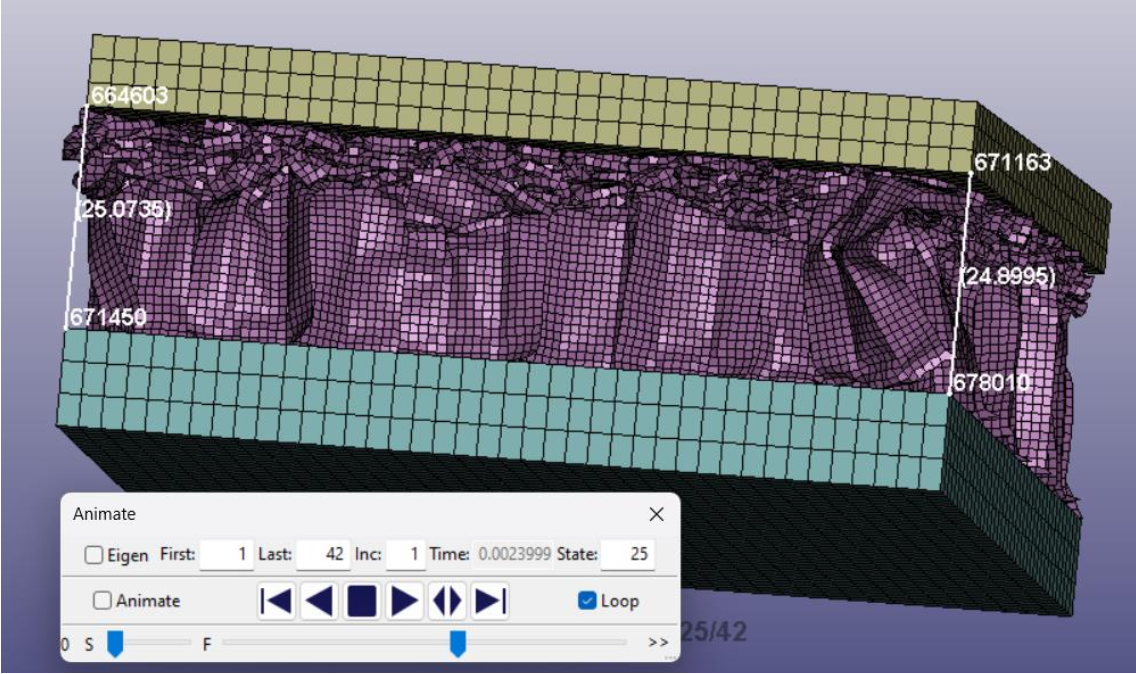
Simulation: ~25 mm
Experimental: ~22 mm
Good agreement!
Learnings & Reflections
- Decreasing time step and TSSFAC improves accuracy but increases runtime and storage.
- In our case, applying this finer resolution to the actual projectile simulation — which already took about 12 days to run with the initial method (a solid block with the honeycomb material model) — made it impractical and eventually crashed the workstation.
- I’m sure I’m still missing some efficiency tricks and better FEM practices, but this is as far as I could push it with my current understanding.
Still, the hands-on simulation experience I gained was invaluable. It has sparked a genuine interest in Computational Mechanics, and I’m sure this foundation will help me greatly as I dive deeper into the theoretical side in the future.
Thanks for reading! Feel free to reach out if you have questions or want to discuss honeycomb modelling and LS-DYNA simulations.